ZOOpt


ZOOpt is a python package for Zeroth-Order Optimization.
Zeroth-order optimization (a.k.a. derivative-free optimization/black-box optimization) does not rely on the gradient of the objective function, but instead, learns from samples of the search space. It is suitable for optimizing functions that are nondifferentiable, with many local minima, or even unknown but only testable.
ZOOpt implements some state-of-the-art zeroth-order optimization methods and their parallel versions. Users only need to add serveral keywords to use parallel optimization on a single machine. For large-scale distributed optimization across multiple machines, please refer to Distributed ZOOpt.
Citation: Yu-Ren Liu, Yi-Qi Hu, Hong Qian, Yang Yu, Chao Qian. ZOOpt: Toolbox for Derivative-Free Optimization. CORR abs/1801.00329 (Features in this article are from version 0.2)
Installation
ZOOpt is distributed on PyPI and can be installed with pip:
$ pip install zoopt
Alternatively, to install ZOOpt by source code, download this project and sequentially run following commands in your terminal/command line.
$ python setup.py build
$ python setup.py install
A simple example
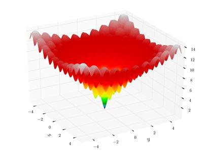
We define the Ackley function for minimization (note that this function is for arbitrary dimensions, determined by the solution)
import numpy as np
def ackley(solution):
    x = solution.get_x()
    bias = 0.2
    value = -20 * np.exp(-0.2 * np.sqrt(sum([(i - bias) * (i - bias) for i in x]) / len(x))) - \
            np.exp(sum([np.cos(2.0*np.pi*(i-bias)) for i in x]) / len(x)) + 20.0 + np.e
    return value
Ackley function is a classical function with many local minima. In 2-dimension, it looks like (from wikipedia)
Then, use ZOOpt to optimize a 100-dimension Ackley function:
from zoopt import Dimension, Objective, Parameter, Opt

dim = 100  # dimension
obj = Objective(ackley, Dimension(dim, [[-1, 1]]*dim, [True]*dim))
# perform optimization
solution = Opt.min(obj, Parameter(budget=100*dim))
# print the solution
print(solution.get_x(), solution.get_value())
# parallel optimization for time-consuming tasks
solution = Opt.min(obj, Parameter(budget=100*dim, parallel=True, server_num=3))
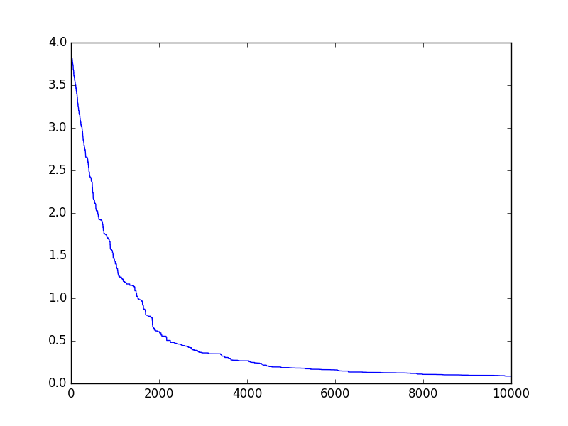
For a few seconds, the optimization is done. Then, we can visualize the optimization progress
import matplotlib.pyplot as plt
plt.plot(obj.get_history_bestsofar())
plt.savefig('figure.png')
which looks like
We can also use ExpOpt to repeat the optimization for performance analysis, which will calculate the mean and standard deviation of multiple optimization results while automatically visualizing the optimization progress.
solution_list = ExpOpt.min(obj, Parameter(budget=100*dim), repeat=3, plot=True, plot_file="progress.png")
for solution in solution_list:
    print(solution.get_x(), solution.get_value())
More examples are available in the EXAMPLES part.
Releases
- Add a parallel implementation of SRACOS, which accelarates the optimization by asynchronous parallelization.
- Users can now set a customized stop criteria for the optimization
- Add the noise handling strategies Re-sampling and Value Suppression (AAAI’18), and the subset selection method with noise handling PONSS (NIPS’17)
- Add high-dimensionality handling method Sequential Random Embedding (IJCAI’16)
- Rewrite Pareto optimization method. Bugs fixed.
- Include the general optimization method RACOS (AAAI’16) and Sequential RACOS (AAAI’17), and the subset selection method POSS (NIPS’15).
- The algorithm selection is automatic. See examples in the example fold.- Default parameters work well on many problems, while parameters are fully controllable
- Running speed optmized for Python